How to Track AI Visibility, and How to Read What It Tells You
The trackers solved collection and left interpretation alone. The record schema, the sampling trade, the null distribution, and whether your design could see a win.
Citon41 min read
Short answer
How do you track AI visibility?
Track AI visibility by recording four nested observations per answer, not one score: whether the brand was named, whether anything was cited, whether the citation was your own domain, and whether that page was the source the answer leaned on. Ask each query several times rather than once, because assistant answers are not stable between identical asks. In our own run, 12 queries asked 5 times each on one model in one day produced 7 that changed outcome with nothing altered between runs. Turn the repeats into a proportion per query, hold half the query set back unworked, and before believing any difference, reshuffle the arm labels a few thousand times to see what a difference looks like when nothing was done. Across 20,000 such splits of our own set with no intervention applied, the null centred on zero with a standard deviation of 0.215, which is the bar a real result has to clear.
Every tool in this category sells you a number. You open the dashboard, you see a visibility score, and the score moves. The thing nobody sells you, and the thing this post is about, is the procedure that turns that movement into a claim you can defend when someone asks how you know.
We ran the cheapest possible version of that check on our own work. Twelve money queries, five identical repeats each, one model, one day, nothing changed between runs. Sixty calls, all sixty succeeded. Seven of the twelve queries changed outcome between identical asks. Not between Tuesday and Friday. Between two asks a few seconds apart with the same words.
That single result is why a procedure exists at all. If more than half your queries disagree with themselves under repetition, then a dashboard reading taken once is a coin flip wearing a decimal point, and the entire question of whether your work moved anything is unanswerable until you have decided how many times to ask.
What follows is the runbook. Nine steps, in order, each one a decision you have to make explicitly because the default is worse than any choice you would make deliberately. Then the proof step, which is the half nobody publishes: how you tell a real move from the noise the system produces on its own.
The short version
A visibility score is a summary of a summary and it is not invertible, so a flat number is consistent with two large opposite movements underneath it. Record four nested observations rather than one boolean, ask each query several times because identical asks disagree, turn repeats into a proportion, hold half the set back, and check any difference against the distribution your own label shuffles produce. Then check whether your design could have detected a plausible win at all, because an underpowered null reads exactly like a failure and is not one.
None of what follows requires a vendor, and none of it is novel statistics. It is the ordinary apparatus of a controlled measurement, applied to an instrument that happens to be an assistant rather than a scale. What makes it worth writing down is that the category has grown up around the collection problem, which is genuinely hard, and has left the interpretation problem almost entirely alone. Collection gives you rows. Interpretation is what turns rows into a sentence you can say to a finance team without hedging.
Before step one, decide which question you are answering
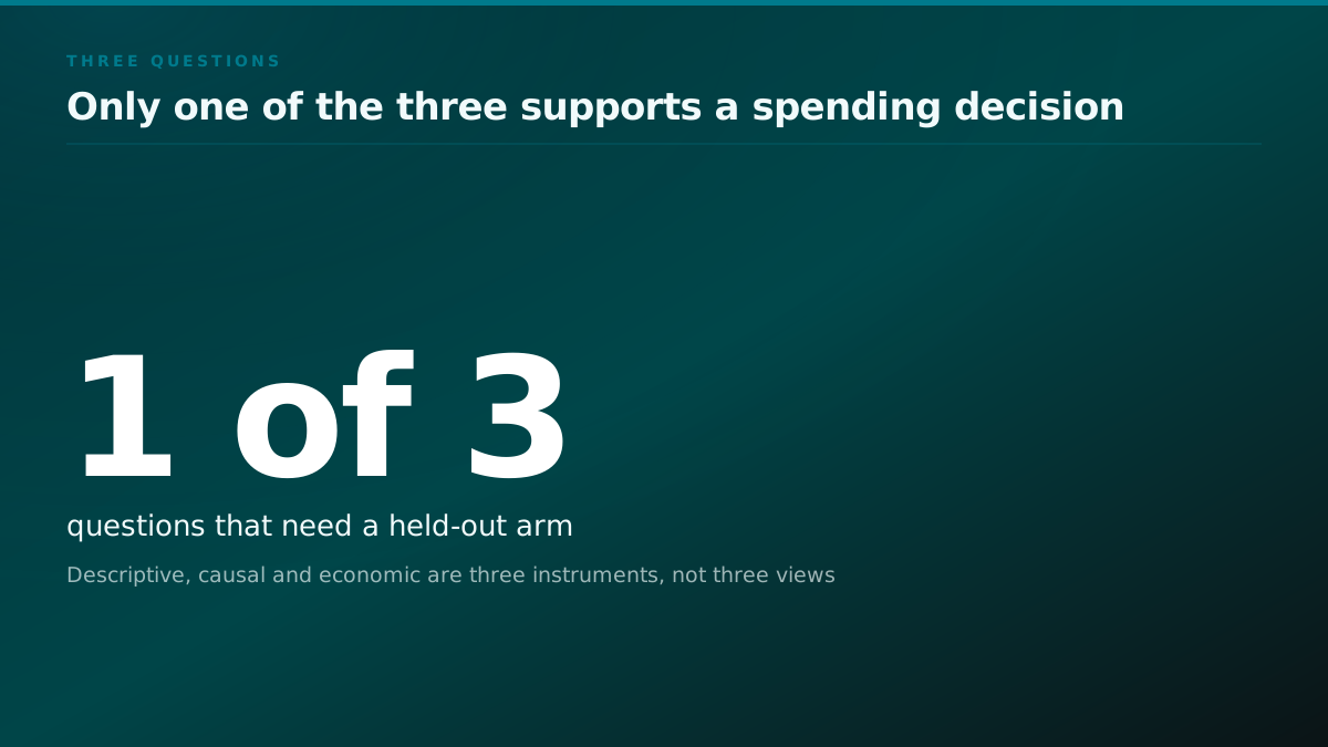
Three questions get called "tracking AI visibility" and they need three different instruments. Picking the wrong one is the most expensive mistake available here, because the setup cost lands months before the mismatch shows up.
Am I visible at all? A descriptive question. One reading, a decent query set, no control, no repeats beyond what stops the number bouncing. This is genuinely cheap and it is the right first purchase. It tells you where you stand and nothing about why.
Did what I did cause the change? A causal question. Needs a held-out arm, a frozen set, a fixed window and a null distribution. This is roughly ten times the setup of the first question and it is the only one that supports a spending decision.
Should I keep paying for this? An economic question, and it sits on top of the causal one. It needs the causal answer plus a cost per unit of movement plus some view of what that movement is worth. Most teams try to answer it directly from the descriptive instrument, which is how a flat quarter gets a programme cancelled and a lucky quarter gets it renewed.
At a glance
Three questions get called tracking, and they need three instruments
| The question | What it needs | What it supports |
|---|---|---|
| Am I visible at all? | One reading, a decent query set, enough repeats to stop the number bouncing. | A description of where you stand. Nothing about why. |
| Did what I did cause the change? | A frozen set, a held-out arm, a fixed window, and a null distribution to read the difference against. | A spending decision. This is the only one that does. |
| Should I keep paying for this? | The causal answer, plus a cost per unit of movement, plus a view of what that movement is worth. | A renewal. Most teams try to answer it from the first instrument, which is how a flat quarter cancels a working programme. |
The runbook below builds the second instrument, because the first is a subset of it and the third is unanswerable without it. If all you need is the descriptive answer, stop after step five and save yourself the control arm.
Why the category defaults to the first question
Not conspiracy, economics. The descriptive instrument is cheap to build, demos well, and produces a chart that moves. The causal one requires deliberately not working half your queries for ninety days, which is a hard thing to sell and a harder thing to keep, and it produces a single number at the end rather than a line that goes up every week.
Across the 64 companies in our own audit of this category, 0 published the number that separates what a team did from what the system did on its own. That is not sixty four failures of rigour. It is a market that has settled on the question that is easiest to answer.
A market does not settle on the easiest question by conspiracy. It settles there because the easiest question is the one that demos well, and deliberately not working half your queries for a quarter does not demo at all.
What you are actually measuring, and why it is four things
Start here, because almost every tracking setup we have looked at collapses four different observations into one field and then wonders why the number is unstable.
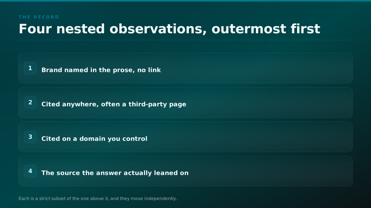
Ask an assistant a buying question. Four things can happen to your brand in the answer it returns, and they are nested inside each other.
The brand can be named. Your product appears in the prose. There is no link, no source card, no attribution. A reader sees your name. A crawler comparing the answer to your site sees nothing connecting them.
It can be cited. The answer carries a source list, or an inline superscript, and one of those sources is a URL. That is a citation. Note that a citation does not have to be your domain. A large share of the citations that carry a brand point at a review site, a forum thread, or a competitor's comparison page that happens to mention you.
It can be cited on your own domain. Now the source is a page you control. This is the subset most people think they are measuring when they say visibility, and it is much smaller than the subset above it.
It can be the load-bearing source. The answer's substantive claim traces to that page rather than to one of the other five sources listed beside it. This is the innermost set, it is the one that actually moves a purchase, and no commercial tool we know of reports it, because separating a decorative citation from a load-bearing one requires reading the answer against the source rather than counting URLs.
On a 40-answer sample that might read 26 named at 65 percent, 14 cited at 35 percent, 6 on your own domain at 15 percent, and 2 load-bearing at 5 percent. Those four are not four metrics. They are one observation with four nested truth values, and the reason that distinction matters operationally is that they move independently and in opposite directions. A month of community work can raise mentions sharply while your own-domain citations sit flat, because the mentions are arriving through third-party pages. A technical fix to your documentation can raise own-domain citations while mentions do not move at all, because the assistant was already naming you and has now simply changed which URL it hangs the name on.
If your tracker stores a single boolean called cited, you cannot tell those two months apart. You will report one as a success and the other as a failure, or the reverse, and you will be wrong roughly half the time in a way no amount of extra sampling can fix, because the information was discarded at write time.
So the first rule of the procedure is a schema rule, not a statistics rule. Record all four. It costs you three extra columns.
The score is a summary of a summary
Commercial dashboards report a share of voice, a visibility index, or a presence percentage. Each of those is a weighted collapse of the four observations above, across some query set you did not choose, at some sampling rate the vendor does not publish, on some assistant mix that changes when the vendor adds a model.
None of that is dishonest. It is what a summary is for. But a summary has one property that matters enormously here: it is not invertible. Given the score, you cannot recover which of the four things moved, on which queries, on which assistant. And since the four move independently, a flat score is entirely consistent with two large opposite movements underneath it.
We have written before about why a single AI visibility score is noise. This post is the constructive half. The argument there was that the number is unreliable. The argument here is that the fix is not a better number, it is a record you can go back to.
Four nested observations, and what each one costs you to skip
| Observation | What it adds | What a tracker usually does | Source |
|---|---|---|---|
| Brand named | Your name appears in the prose. No link, no source card. | Counts it as a mention and stops. | unknown |
| Cited anywhere | The answer carries a source, which is frequently not your domain. | Collapses it into the same field as a mention. | unknown |
| Cited on your own domain | The source is a page you control. | Reports this as the headline number when it reports it at all. | unknown |
| The load-bearing source | The answer's substantive claim traces to that page. | Does not report it. Separating a decorative citation from a load-bearing one needs the answer read against the source. | unknown |
as of 2026-09-01
Method: The four levels are a schema proposal, not a measurement, and they are tagged unknown for that reason. What would falsify the schema is finding a fifth distinction that moves independently of these four, or showing that two of them never diverge in practice, either of which would be worth knowing.
A visibility score reports somewhere in the top two bands.
The bottom band is the one a buyer acts on. No commercial tool reports it.
The four move independently and sometimes in opposite directions, so a single stored boolean cannot tell a month of third-party mentions apart from a month of owned-page citations. Recording all four costs three columns.
Step 1, the query set, in one paragraph
We have published the construction rules elsewhere and there is no point restating them: choose around forty unbranded buyer questions, never questions carrying your own brand name, never questions you already win, write the list down in week zero and do not edit it. That is covered in LLM SEO, what it actually is and what the work looks like, along with the two ways the set gets chosen to flatter.
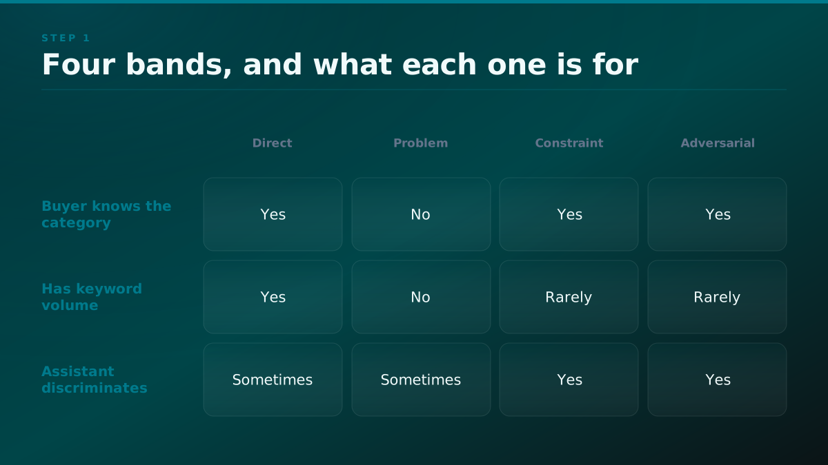
One thing that post does not do is tell you to record which KIND of question each one is, and you want that field because you will read the bands separately later. Four bands: direct comparison, where the category is named and a recommendation asked for; problem-shaped, where the pain is described but the category is not, which is where a category-creating product lives and which has no keyword volume by construction; constraint-shaped, the same question with a budget or a stack attached, which is where an assistant actually discriminates rather than listing five; and adversarial, the questions a sceptical prospect asks, which nobody wants to measure and which decide the deal.
One column. It costs nothing at write time and it is unrecoverable afterwards.
Step 1
Four bands, recorded as a field rather than kept in someone's head
- Frozen query setAround forty unbranded buyer questions, written in week zero and not edited.
- Direct comparisonThe category is named and a recommendation asked for. Highest intent, smallest band.
- Problem-shapedThe pain described without the category. No keyword volume by construction.
- Constraint-shapedThe same question with a budget or a stack attached, where an assistant actually discriminates.
- AdversarialWhat a sceptical prospect asks. Nobody wants to measure these and they decide the deal.
- Frozen query setDirect comparisonband
- Frozen query setProblem-shapedband
- Frozen query setConstraint-shapedband
- Frozen query setAdversarialband
Step 2, choose the repeat count
This is the decision the rest of the procedure is built on, and the reason it is hard is that your measurement budget is one number and every dimension you add spends it.
You have some number of assistant calls you can afford per week. Call it a budget. That budget is consumed multiplicatively: queries times repeats times assistants times readings per week. Raising any one of those four lowers the others, and the total is conserved.
Most teams spend the whole budget on the first dimension. They track two hundred queries once each per week, across three assistants, and feel thorough. What they have actually built is an instrument with a repeat count of one, which means every reading has an unknown error bar, which means no difference between two readings can be interpreted.
Our own step-zero run is the argument for spending differently. Twelve queries, five repeats, one model, one day: seven of the twelve flipped outcome across identical asks. If we had run those twelve queries once each, we would have recorded twelve booleans and had no way of knowing that seven of them were unstable. The instability is only visible because the repeats are there. A single-repeat design does not produce a noisy reading, which would at least be honest. It produces a confident reading with the noise hidden inside it.
How to pick the number
The repeat count you need is a function of how unstable your queries are, and you do not know that until you measure it, so the procedure is two-phase.
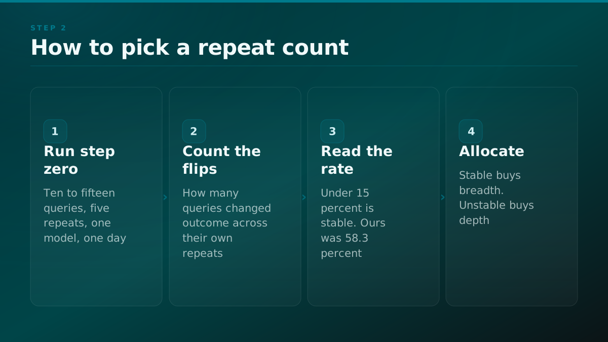
Phase one, step zero. Take a small set, ten to fifteen queries, run each of them five times on one model on one day, changing nothing. Count how many queries returned a different outcome across their own repeats. That fraction is your instability rate, and it is the most useful number you will produce in the first month.
Phase two, allocate. If your instability rate is low, say under 15 percent, 3 repeats is defensible and you can spend the rest of the budget on breadth. If it is high, and ours was 58.3 percent, 7 of 12, breadth is the wrong purchase. Five repeats minimum, and you should consider whether a smaller query set measured properly beats a larger one measured once.
The uncomfortable implication, which is why almost nobody publishes this step, is that a correctly-sampled tracker covers far fewer queries than an incorrectly-sampled one, and looks worse in a feature comparison for exactly that reason.
Two allocations of one 600-call weekly budget
| Allocation | Queries | Repeats | Engines | Can it separate a move from noise | Source |
|---|---|---|---|---|---|
| Breadth | 200 | 1 | 3 | No. No query carries an error bar, so no difference is readable. | derived |
| Balanced | 40 | 5 | 3 | Yes, for a large effect. This is the usual compromise. | derived |
| Depth | 15 | 40 | 1 | Yes. Fewest queries, and the only one whose per-query estimate is tight. | derived |
n = 600 · as of 2026-09-01
Method: Derived arithmetic, not a measurement: queries times repeats times engines against a fixed 600-call weekly budget, with the readable column judged against our own measured instability rate of 7 of 12 queries flipping between identical asks. Falsify it by measuring a lower instability rate on your own set, which moves the readable threshold left.
1 repeat per query, so no query has an error bar at all
5 repeats per query, so each query carries its own error bar
20 calls either way
Same spend, same week, same engine. Only the second allocation can tell a move from noise, and our own step zero run is the reason: 12 queries asked 5 times each, 7 of them changed outcome with nothing altered between runs.
Step 3, engine coverage, and what to do when they disagree
Report engines separately, never blended. That rule is already published and the reasoning behind it is not repeated here.
What is not published anywhere is the question it leaves open, and it is the one that actually comes up: what do you do when the treated arm wins on one engine and loses on another?
You have two results, not one confused result, and you report both. A cross-engine disagreement is information about the engines rather than a failure of the measurement. One of them is retrieving from an index that has your new page and one is not, or one weights a third-party source you never touched. Averaging them to resolve the discomfort throws away the only interesting thing in the reading.
The sizing consequence is the part people miss. Engines multiply your call budget before anything else does, so decide the count first and pick the smallest number you can afford to sample properly. A well-sampled reading of one engine supports a claim. Four badly-sampled readings support none and cost four times as much.
Step 3
One design, replicated per engine, never blended
- Frozen query setThe same questions, asked identically everywhere.
- Engine A runIts own baseline, its own arms, its own null distribution.
- Engine B runSame, and independent. It may disagree with A.
- Two resultsReported side by side. A disagreement is information about the engines.
- Frozen query setEngine A runasked
- Frozen query setEngine B runasked
- Engine A runTwo resultsits own null
- Engine B runTwo resultsits own null
Comparison
Three ways to spend a fixed budget across engines
| All four engines | Two engines | One engine, sampled properly | |
|---|---|---|---|
| Repeats per query at a fixed budget | Roughly a quarter of what one engine would get. | Half. | All of it, which is the only column where a per-query estimate is tight. |
| What a difference means | Unreadable on any single engine. | Readable only for a large effect. | Readable, and attributable to one retrieval behaviour. |
| What you can say afterwards | Something moved somewhere. | Something moved on one of two. | This engine moved by this much, against this null. |
| What you give up | Nothing, and you learn nothing. | Coverage of two engines. | Coverage of three engines, which is a real loss and is the honest cost. |
Step 4, the record schema
Here is the whole thing. Every run writes one row.
The row carries: the query id, the query band, the run timestamp, the assistant and the model version string if the API exposes one, the repeat index, the four nested observations from the opening section, the full answer text, the full source list as returned, and a boolean for whether the assistant performed a live retrieval on this call if that is observable.
Two of those fields are the ones people skip and both are the ones you will need most.
Store the full answer text. It is the only thing that lets you go back and re-derive a metric you did not think of at the time. Six weeks in you will want to know whether the assistant described you accurately, or whether a competitor was named alongside you, or whether a specific objection surfaced. Every one of those is a re-read of stored text and none of them is possible from a stored boolean.
Store the model version string. Assistants get silently upgraded. A step change in your numbers that lines up with a version change is a measurement artefact, and without the version field you will spend a week attributing it to your own work.
The row you write on every call
| Field | Why it is there | Source |
|---|---|---|
| query_id, band | Lets you read the bands separately later. One column, unrecoverable afterwards. | derived |
| run_ts, repeat_index | A proportion needs a denominator. Without the index there is none. | derived |
| engine, model_version | The only way to tell a silent provider upgrade from your own success. | derived |
| arm | Stamped per call, so the assignment cannot be edited after the fact. | derived |
| named, cited, own_domain, load_bearing | The four nested observations, stored separately. | derived |
| retrieved | Whether a live retrieval happened on this call, where that is observable. | derived |
| sources_raw | The array exactly as returned. Parse downstream, never at write time. | derived |
| answer_text | The whole answer. This is the field people cut, and the one that makes every future question answerable. | derived |
as of 2026-09-01
Method: Derived from the failure modes we have hit rather than from a standard. Each field is here because its absence broke a specific reading. Falsify it by naming a question you later needed to answer that none of these fields supports, which is exactly how the list grew.
Two things not to store as your primary key
Do not key on rank position. Assistant answers are not ranked lists, and where a source appears in a citation array is not consistently meaningful across surfaces. A source list is frequently ordered by retrieval order rather than by importance.
Do not key on a similarity score between the answer and your page. It is cheap to compute and it feels rigorous, and it will move for reasons unconnected to whether you were cited, because the assistant rephrases.
What a single row of the log looks like
Step four described the schema in prose. Here it is as an object, because a schema you can copy is worth more than a schema you agree with.
The record
One row per call, and the six fields that do non-obvious work
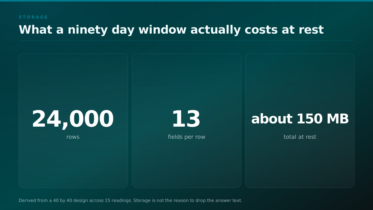
24,000
Rows, 90-day window
13
Fields per row
2 to 6 KB
Answer text stored
about 150 MB
Total at rest
- model_version, stamped per call
- arm, stamped per call rather than looked up later
- repeat_index, so a proportion has a denominator
- sources_raw, the array exactly as returned, parsed downstream
- answer_text, the whole answer
- A revenue fieldThere is none. This instrument does not observe the path from a citation to a deal, and a column implying otherwise would be the overclaim the post argues against.
Six fields in that row do work that is not obvious.
model_version is the only thing that lets you detect the mid-window model change that the whole design is most vulnerable to. Without it, a silent upgrade is indistinguishable from your own success.
arm is stamped per call rather than looked up later, because an arm assignment stored only in a separate table is an arm assignment that can be edited after the fact.
repeat_index is what makes a proportion computable. A row without it is a row you cannot put a denominator under.
retrieved records whether the assistant performed a live retrieval on this call where that is observable. A brand named from training data and a brand named from a retrieved page are different events with different levers, and only one of them responds to publishing a page this month.
sources_raw is the full array as returned, unparsed. Parse it downstream. Parsing at write time bakes today's understanding of the response shape into a record you will want to re-read in six months.
answer_text is the whole answer. This is the field people cut to save storage and it is the one that makes every future question answerable.
Storage, since that is the objection
A 90 day run at the sizes above produces on the order of 24,000 rows. Answer text runs 2 to 6 kilobytes each, so call it 150 megabytes at the top of that range, which is nothing, and it is the difference between a measurement you can interrogate and a chart you have to trust.
Step 5, normalisation, turning runs into a reading
You now have rows. A reading is a function that turns a week of rows into one number per query, and this function needs to be written down once and never quietly changed, because changing it re-writes your history.
The unit we would defend is: for each query, the proportion of its repeats in which the observation was true, at each of the four nesting levels. Twelve queries at five repeats gives you, per level, twelve proportions each drawn from five trials. That is the reading.
That formulation has three properties worth stating.
It preserves the denominator. A query answered in three of five repeats is different from a query answered in five of five, and both are different from a query answered in one of five, and a boolean throws all three into two buckets.
It is aggregatable without lying. The mean of twelve proportions is a defensible summary because each proportion is on the same scale with the same denominator.
It surfaces instability directly. A proportion sitting near one half is, by construction, a query that disagrees with itself, which is exactly what you want flagged rather than averaged away.
A worked reading, with the arithmetic in the open
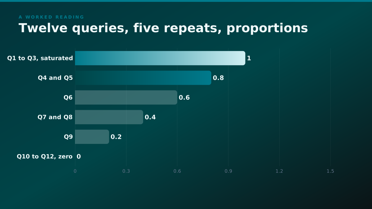
Twelve queries, five repeats, one engine, one week. Sixty calls.
Suppose the outcome at the cited-on-your-domain level comes back like this: three queries hit on all five repeats, two hit on four, one on three, two on two, one on one, and three never hit at all. Twelve proportions: 1.0, 1.0, 1.0, 0.8, 0.8, 0.6, 0.4, 0.4, 0.2, 0, 0, 0.
The reading is the mean of those twelve, which is 0.517. Not "52 percent visibility". The mean of twelve per-query proportions, each drawn from five trials, at one nesting level, on one engine, in one week.
Three things are now visible that a single number would have hidden. Three queries are at zero, which is a content gap rather than a ranking problem. Three queries are at 1.0, which means they are saturated and cannot contribute to any future lift, so working them is wasted effort. And four queries sit between 0.2 and 0.6, which is where the instability lives and where a second week will disagree with this one.
That last group is the actionable one, and it is also the one that will make your arm mean bounce. If you want a quieter instrument, the lever is more repeats on those four, not more queries overall.
Twelve queries, five repeats, one engine, one week
| Query | Repeats hit | Proportion | What it tells you | Source |
|---|---|---|---|---|
| Q1 to Q3 | 5 of 5 | 1.0 | Saturated. Cannot contribute to any future lift, so working them is wasted effort. | unknown |
| Q4, Q5 | 4 of 5 | 0.8 | Strong and slightly unstable. | unknown |
| Q6 | 3 of 5 | 0.6 | Unstable. Will disagree with itself next week. | unknown |
| Q7, Q8 | 2 of 5 | 0.4 | Unstable, and the actionable group. | unknown |
| Q9 | 1 of 5 | 0.2 | Marginal presence. | unknown |
| Q10 to Q12 | 0 of 5 | 0.0 | A content gap rather than a ranking problem. | unknown |
| Reading | 31 of 60 | 0.517 | The mean of twelve per-query proportions. Not a visibility percentage. | derived |
n = 60 · as of 2026-09-01
Method: An illustrative distribution chosen to show the three groups a single number hides, with the final row derived arithmetically from the rows above it. The per-query outcomes are unknown rather than measured because they are an example and not a run. The arithmetic is checkable: the twelve proportions sum to 6.2 and 6.2 divided by 12 is 0.517.
The trap in weighting by volume
There is a strong pull toward weighting queries by search volume, so the reading reflects business value. Resist it for the primary reading, and here is the specific reason.
Volume figures for assistant queries do not exist. The volumes you would weight with are keyword volumes from a search index, attached to strings that are not the strings you are measuring. Weighting a set of full-sentence buying questions by the volumes of the short keywords they resemble imports an entirely different distribution into your reading, and it does it invisibly.
Keep a weighted view if it is useful commercially. Keep the unweighted proportion as the instrument.
Step 5
From calls to a reading, in three steps that must never change mid-programme
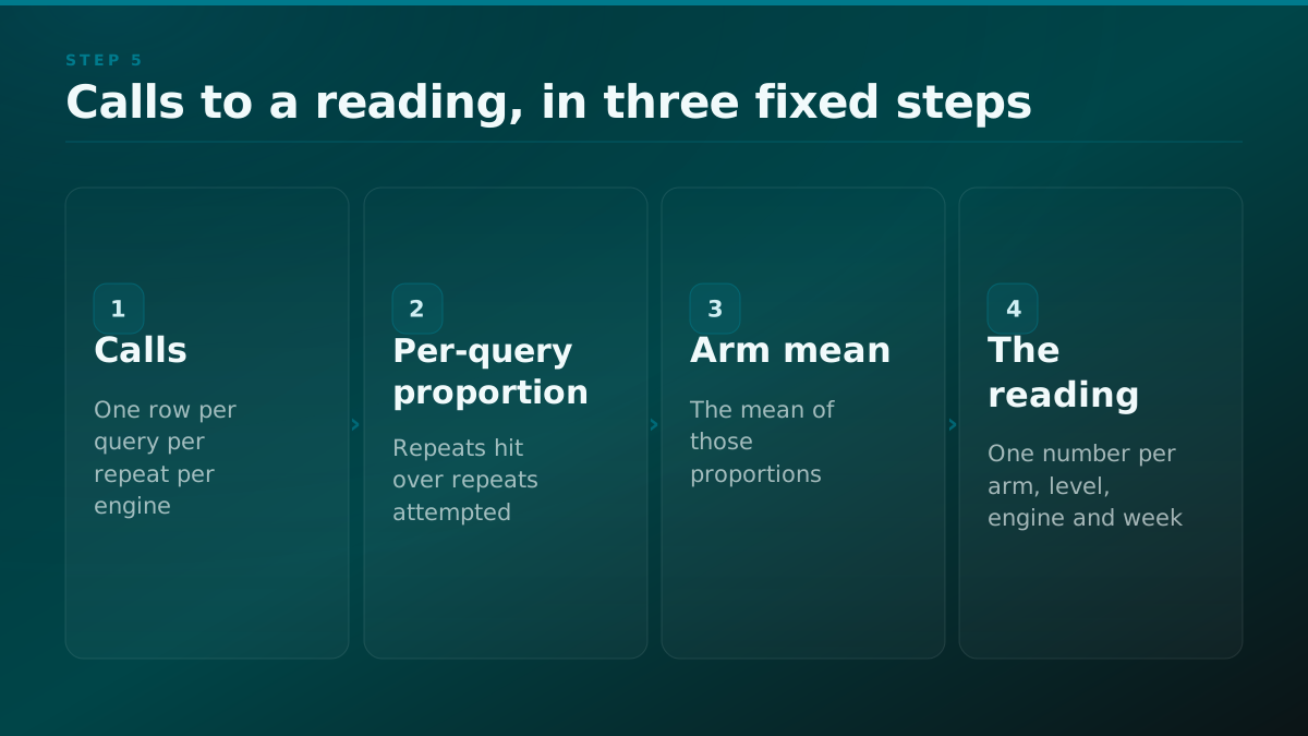
- CallsOne row per query per repeat per engine, with the four observations stored separately.
- Per-query proportionRepeats hit divided by repeats attempted, at one nesting level.
- Arm meanThe mean of those proportions. Same scale, same denominator, aggregatable without lying.
- The readingOne number per arm per level per engine per week.
- CallsPer-query proportiongroup by query
- Per-query proportionArm meanmean
- Arm meanThe readingper level, per engine
Step 6, the baseline
A baseline is not a reading. It is a distribution.
This is the step that separates a tracker from a measurement, and it follows directly from step two. If your queries disagree with themselves, then a single week's reading is one draw from a distribution, and you need to know the width of that distribution before any later reading means anything.
So: before you touch anything, take the baseline reading at least three times, on separate days, with the query set frozen and no work done in between. You now have three readings that differ only by noise, which gives you a first, crude estimate of how much this instrument moves on its own.
That estimate is the number you will hold every subsequent claim against. If your three no-work readings span four percentage points, then a subsequent five point move is barely outside your own noise, and calling it a win is a coin flip.
Why the baseline is three readings and not one
| What you take | What you learn | What you still cannot say | Source |
|---|---|---|---|
| One reading | Where the number sat on one day. | Whether a later move is larger than the instrument's own week-to-week wobble. | derived |
| Three readings, no work done | A crude estimate of the spread the instrument produces on its own. | Whether a move was caused by you. That needs the held-out arm. | derived |
| Three readings plus a held-out arm | The spread, and a comparison that subtracts whatever the system did by itself. | Anything about revenue, which this instrument does not observe. | derived |
as of 2026-09-01
Method: Derived from the design, not measured on a client. The claim that one reading is insufficient rests on our own measured instability, 7 of 12 queries flipping between identical asks. Falsify it by running three no-work readings and finding them identical, which would mean your queries are stable and one reading is enough.
Why one baseline reading feels sufficient and is not
The intuition that betrays people here is that a baseline is a starting position, like a weight on a scale. It is not, because the scale is not stable. It is closer to a measurement of a moving object with a shaky instrument, where you need several readings just to establish where the object currently is.
Our own repeat data is the compact version of this argument. Seven of twelve queries flipped between identical asks on one model in one day. A baseline taken from one pass across those twelve queries would have recorded seven values that had a roughly even chance of being their own opposite.
Step 7, the held-out arm, in one paragraph
Split the frozen set, work one half, deliberately do not work the other, measure both across the same window. The design, what it costs to run, and the failure where somebody quietly starts working the held-out arm in week six, are all covered in the post linked above.
Three operational details that are not.
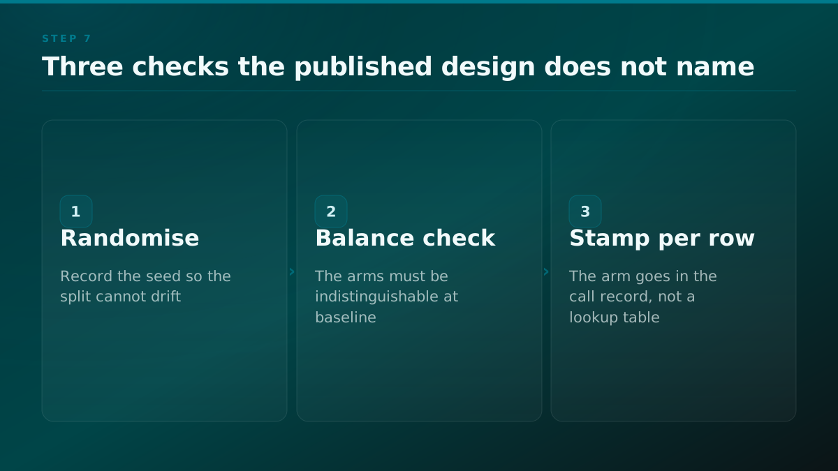
Randomise the split and record the seed. A hand-made split is informed by your sense of which queries you can win, and that sense is correlated with the outcome, so the split itself manufactures the difference the experiment then measures. Record the seed so the assignment is reproducible and cannot drift.
Check the arms are balanced at baseline. Before day zero, compare the two arms on the baseline readings. They should be indistinguishable. If they are not, you drew an unlucky split, and you re-draw it now rather than discovering at week thirteen that your arms started apart.
Stamp the arm on every row. An assignment stored only in a separate lookup table is an assignment that can be edited after the fact. Write it into the call record.
Step 7
The three operational details that are not in the published design
- Frozen setAround forty unbranded questions, already written down.
- Randomised splitSeed recorded, so the assignment is reproducible and cannot drift.
- Baseline balance checkThe arms must be indistinguishable before day zero. Re-draw if not.
- Arm stamped per rowWritten into the call record, not held in a lookup table that can be edited.
- Frozen setRandomised splitseed recorded
- Randomised splitBaseline balance checkbefore day zero
- Baseline balance checkArm stamped per rowthen freeze
Step 8, the proof step
You have two arms, a worked half and an unworked half, and a difference between them. The question that decides whether you have a result is: how big a difference would you have seen if you had done nothing at all?
Most teams answer this by intuition, and intuition is badly calibrated here because the noise is large and structured. The answer you want is empirical, and it is cheap to compute because you already have the data.
Reshuffle the labels
Take your query set and its outcomes for the window. Now throw away the real worked and unworked labels, and assign the labels at random. Compute the difference between the two arms under that fake assignment. Do it again. Do it twenty thousand times.
What you get is a distribution of differences produced by an experiment in which, by construction, nothing was done. That is the shape of your own noise. Your real difference either sits inside that shape, in which case it is indistinguishable from having done nothing, or it sits out in the tail, in which case you have a result.
We ran exactly this on our own query set. Twenty thousand random splits, no intervention applied at all, and the difference between the two halves centred on zero: mean plus or minus 0.0016, standard deviation 0.215.
Two things in that result are worth pulling apart, because they say opposite things and both matter.
The mean is essentially zero, which is the good news. It means the two-arm design is unbiased. If it had come back centred somewhere other than zero, the instrument itself would have been manufacturing a difference, and every reading it ever produced would have been contaminated. This is a kill test for the design, and the design passed it.
The standard deviation is 0.215, which is the sobering news. That is the width of the noise. A difference between arms has to clear a substantial multiple of that spread before it stops being explainable by the shuffle. A small observed difference is not a small result. It is not a result.
Our own null distribution, 20,000 label shuffles
| Quantity | Value | What it means | Source |
|---|---|---|---|
| Random splits | 20,000 | Each one a fake experiment in which, by construction, nothing was done. | measured |
| Mean difference | plus or minus 0.0016 | Essentially zero, which is the design's kill test. A non-zero mean would mean the instrument manufactures a difference. | measured |
| Standard deviation | 0.215 | The width of the noise. This is the bar a real result clears. | measured |
| Conventional threshold | about 0.43 | Two standard deviations. Derived from the row above, not a separate measurement. | derived |
n = 20,000 · as of 2026-09-01
Method: Our own run: 20,000 random splits of our own query set with no intervention applied at all, arm difference recomputed under each fake assignment. The first three rows are measured; the threshold is derived by doubling the measured standard deviation. What would falsify it is a rerun whose mean is not centred on zero, which would invalidate the design rather than the result.
Why this beats a p-value from a stock test
You could run a t-test. The reason we prefer the permutation is that a stock test carries assumptions about the shape of the underlying distribution, and assistant outcomes are binary, clustered by query, correlated across repeats of the same query, and correlated across queries that share a topic. Those assumptions are wrong in at least three ways here.
The permutation test makes almost no assumptions. It uses your own data to generate its own null, so whatever weird correlation structure your query set has is present in both the real difference and the fake ones. That is the whole trick, and it is why it survives contact with data this messy.
The one thing to be careful about
Shuffle at the level you randomised at. If you assigned whole queries to arms, shuffle whole queries, not individual repeats. Shuffling repeats would break the within-query correlation that exists in your real data, which makes the null distribution artificially narrow, which makes everything look significant.
This is the most common way a permutation test is run wrong, and the failure is silent: you get a beautiful tight null and a triumphant result.
Step 8
The loop that produces your own null
- Observed outcomesOne window of readings, arms and all, exactly as collected.
- Discard the labelsThrow away which arm each query was really in.
- Reassign at randomAt the QUERY level, keeping each query's repeats together.
- Fake differenceCompute the arm difference under this fake assignment. Repeat 20,000 times.
- Null distributionThe shape of a difference produced by doing nothing. Ours: mean plus or minus 0.0016, sd 0.215.
- Observed outcomesDiscard the labelskeep the data
- Discard the labelsReassign at randomquery level
- Reassign at randomFake differencecompute
- Fake differenceReassign at random20,000 times
- Fake differenceNull distributioncollect
From a verdict to an interval
A permutation test answers a yes or no question: is this difference bigger than what shuffling produces. That is the right first question and it is not the last one, because a yes leaves you with a point estimate and no sense of how precise it is.
The interval is the same machinery run the other way, and it takes about ten extra lines.
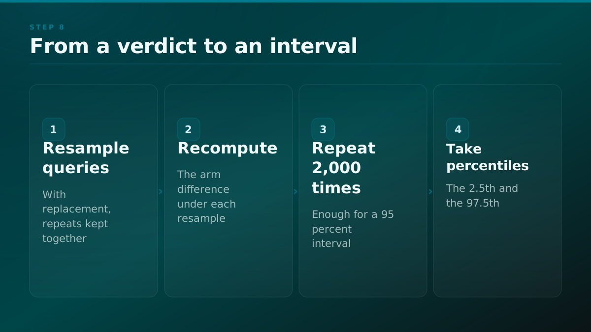
Resample your queries with replacement, keeping each query's repeats together, and recompute the arm difference. Do that 2,000 times, which is enough for a 95 percent interval and takes seconds. Sort the resulting differences and take the values at the 2.5th and 97.5th percentiles. That pair is your ninety five percent interval, and it is the number to put in the report, because it carries both the size of the effect and how sure you are of it.
Two practical notes. Resample the query, not the repeat, for the same reason you shuffle the query in the permutation: the repeats inside a query are not independent of each other. And expect the interval to be wide on a first run. Wide is honest. A narrow interval on a twelve query pilot would be a sign that something in the resampling has broken the correlation structure.
The four questions to ask before you believe your own reading
Run these in order. Any one of them failing sends you back a step rather than forward to a conclusion.
Did the instrument stay the same? Same query wording, same repeat count, same engine, same normalisation function, same model version. If any of those moved, the comparison is across two instruments.
Did the arms fail equally? Pull the per-arm failure counts. A gap there is an asymmetric shock and it invalidates the window regardless of how good the difference looks.
Is the difference outside the null? Not larger than last quarter. Outside the distribution your own shuffles produced. Roughly 2 standard deviations of that null is the conventional line and, given ours is 0.215 wide, that puts the bar at about 0.43, which is not small.
Could the design have seen a smaller effect? If the answer is no, then a null result tells you nothing and should be reported as inconclusive rather than negative. This is the question that turns a wasted quarter into a resized design.
Four questions to ask before believing your own reading
| Question | How you check it | What a failure means | Source |
|---|---|---|---|
| Did the instrument stay the same? | Same wording, repeat count, engine, normalisation function and model version string. | The comparison is across two instruments, not two weeks. | derived |
| Did the arms fail equally? | Pull the per-arm call failure counts for the window. | An asymmetric shock landed on the comparison. The window is void. | derived |
| Is the difference outside the null? | Compare it against your own shuffled distribution, not against last quarter. | It is indistinguishable from having done nothing. | derived |
| Could the design have seen a smaller effect? | Check the observed difference against your minimum detectable lift. | A null result is inconclusive, not negative. Resize and rerun. | derived |
as of 2026-09-01
Method: Derived from the four ways we have seen a reading misreported. Each row states its own failing result, which is what makes it a check rather than a reassurance. Falsify the list by finding a fifth failure none of the four catches.
From the field
Sixty four companies, zero published attribution numbers
Our own audit of this category looked at 64 companies selling AI-visibility measurement. Not one published the number that separates what a team did from what the system did on its own. That is not 64 failures of rigour. It is a market that has settled on the question that is cheapest to answer, because presence data collects itself and a held-out arm has to be defended internally for a quarter.
A reading here is inside the shuffles. Indistinguishable from having done nothing.
A reading out here clears its own noise. This is what a result looks like.
Our own run: 20,000 random splits of the same query set with no intervention applied, difference between halves centred on zero, mean plus or minus 0.0016, standard deviation 0.215. The mean being zero is what proves the design is unbiased. The spread is what your result has to clear.
Step 9, power, or how many queries you actually need
Power is the question of whether your design could detect a real effect if one were there. It is the step almost everyone skips, and skipping it is how a team runs a three month test, gets a null result, and concludes the work does not function when in fact the instrument was never capable of seeing it.
We ran it on our own pilot design and the answer was uncomfortable. A twelve-query by five-repeat design has a minimum detectable lift of 51.1 percentage points. That is roughly four times underpowered against the design that would actually detect a normal-sized effect.
Read that carefully, because it is the most useful number in this post. It does not say our approach does not work. It says a pilot of that size can only detect an enormous effect, so a null result from it means nothing at all. Anything smaller than a fifty point swing would have been invisible to it, and fifty point swings are not what real work produces.
What the pilot design could and could not have detected
| Property | Value | Consequence | Source |
|---|---|---|---|
| Design | 12 queries by 5 repeats | 60 calls. Cheap, and the right first thing to run. | measured |
| Minimum detectable lift | 51.1 percentage points | Only an enormous effect is visible. | derived |
| Underpowered by | roughly 4x | Against a design that would detect a normal-sized effect. | derived |
| What a null from it means | Nothing | Inconclusive, not negative. Reporting it as negative is the expensive mistake. | derived |
n = 60 · as of 2026-09-01
Method: The design is measured, ours, and ran. The floor and the underpowering factor are derived from the variance in that same run. We publish no causal lift figure because this design could not have measured one, and publishing one off it would be the overclaim this post argues against.
What to do about it
Three levers, in order of cost.
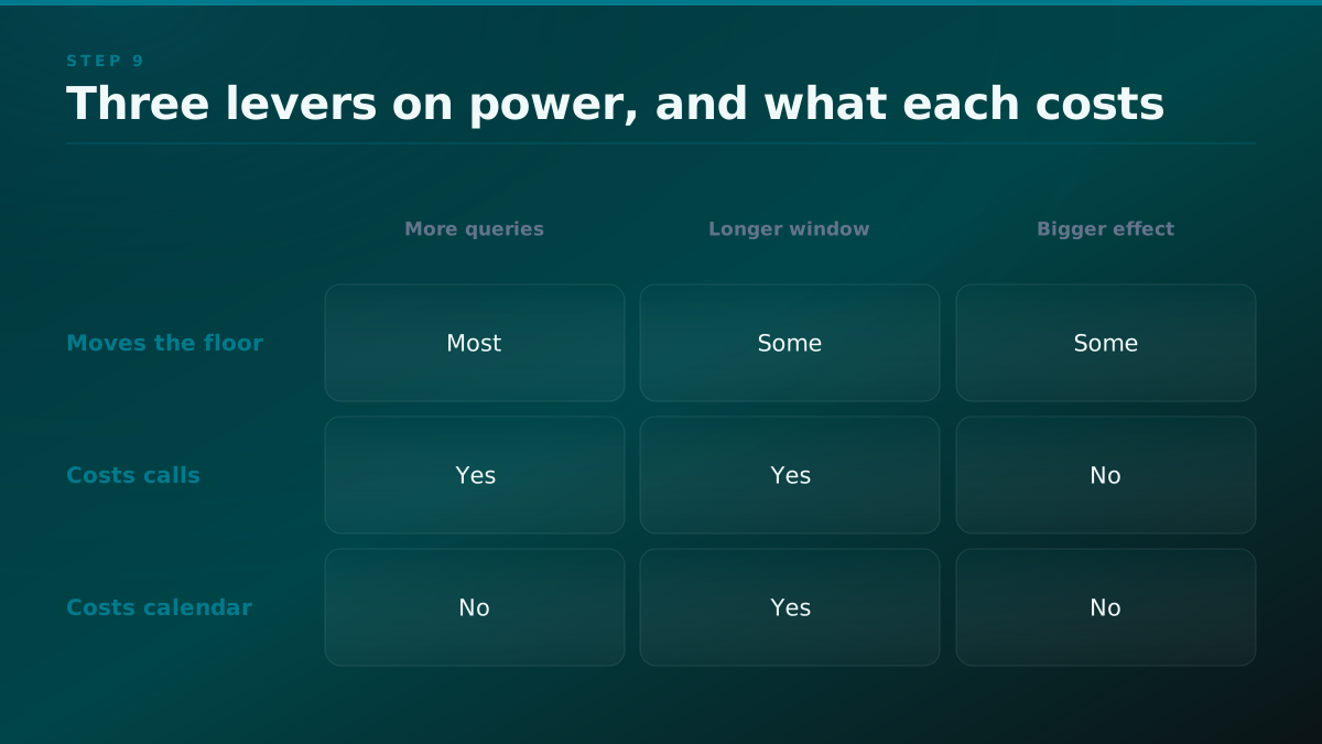
More queries. Power scales with the number of independent units, and the unit is the query, not the repeat. Doubling repeats sharpens each query's estimate; doubling queries adds new independent evidence. If you have to choose, queries win for power and repeats win for stability, which is why the budget conversation at step two is genuinely a trade and not a preference.
A longer window. More readings across the same queries reduce the standard error of each arm's estimate, at the cost of calendar time and of drift in the underlying system.
A larger expected effect. Concentrate the work rather than spreading it. Ten queries worked hard produce a bigger arm difference than fifty worked lightly, and a bigger effect is easier to detect at any given sample size.
The one lever that does not exist is analysing harder. No statistical method will extract a signal a design was not powered to see.
Step 10, the arithmetic that sizes your design
Every number in the previous section is an output. Here is the input, so you can size your own run rather than borrowing ours.
The minimum detectable lift is set by three things: how noisy a single query's outcome is, how many independent queries you have, and how confident you insist on being. The relationship is the ordinary one, which is that the smallest difference you can distinguish from zero shrinks with the square root of your sample size. Quadrupling the queries halves the floor. Nothing else in the design has that leverage.
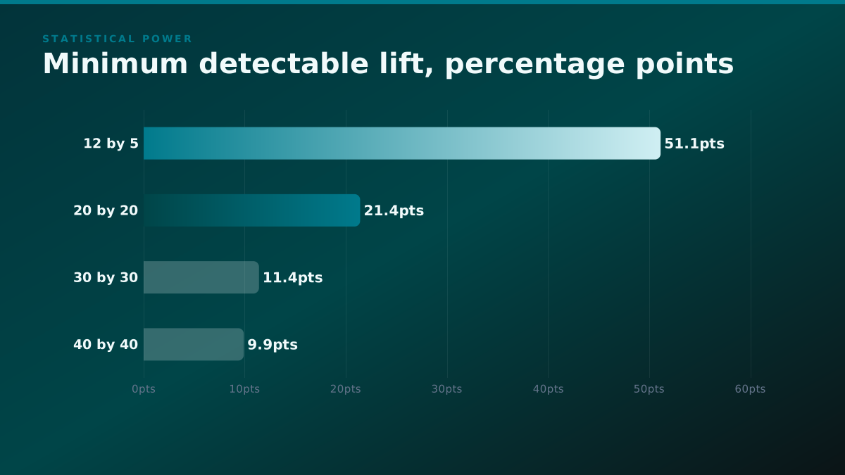
We have published four rungs of that ladder from our own work, and they are worth laying side by side because the spread is larger than people expect: 40 queries by 40 samples puts the floor at 9.9 percentage points, 30 queries at 11.4, 20 queries at 21.4, and the 12 by 5 pilot at 51.1.
Statistical power
Minimum detectable lift by design size
| Point | Value (percentage points) |
|---|---|
| 12 queries by 5 samples | 51.1 percentage points |
| 20 queries by 20 samples | 21.4 percentage points |
| 30 queries by 30 samples | 11.4 percentage points |
| 40 queries by 40 samples | 9.9 percentage points |
Read the bottom rung first. A 12 by 5 pilot cannot see anything smaller than a 51.1 point swing. Now read the top rung. At 40 by 40 the floor is 9.9 points, which is inside the range a real programme might actually produce. Between them sits the rung that matters commercially: at 20 to 30 queries the floor runs 11.4 to 21.4 points, still larger than a plausible real win, so a genuine result at that size comes back as not distinguishable from zero. Going from 20 queries to 40 roughly halves the floor, from 21.4 to 9.9, which is the square-root relationship doing its work.
That is the sentence to hold on to when a vendor quotes a design. A tracker that samples twenty queries is not a smaller version of one that samples forty. It is an instrument that will report your success as a null.
Why the noise term is the one you cannot argue with
The floor is proportional to the spread of your own null distribution, and we measured that at a standard deviation of 0.215 across twenty thousand splits. You do not get to assume a smaller one. If your queries are less unstable than ours, your floor drops, and the way to find out is step zero, not optimism.
This is also the honest answer to why we do not publish a causal lift figure. The instrument exists, its kill test passed, and the pilot that ran on it was underpowered by roughly a factor of four. Publishing a lift number off that design would be publishing a number the design could not have measured.
Step 11, what a call failure does to your arms
Eight times across our published work we have reported that sixty of sixty calls succeeded. What none of that says is what to do when they do not, and this is the operational gap that will bite you in the first month.
A failed call is not a missing value. It is a value that is missing for a reason, and the reason is frequently correlated with the thing you are measuring.
Write down the retry policy before the run. Ours: retry twice with a delay, then record the call as failed rather than substituting anything. A retried call counts as one repeat, not two.
Decide what a partial trial does to its query. If a query gets three of its five repeats, you can either score it on three, which changes its denominator and therefore its weight, or void it. We void it, and record the void, because a mixed-denominator set quietly reweights itself.
Watch the failure rate per arm, and treat asymmetry as a stop condition. This is the one that actually matters. If an engine rate-limits harder on one arm's queries than the other's, you have an asymmetric shock landing on exactly the comparison the whole design rests on, and no amount of sampling repairs it. Report failures per arm in every reading. Equal failure rates are absorbed by the control. Unequal ones invalidate the window.
What to do when a call fails
| Situation | The rule | Why | Source |
|---|---|---|---|
| A call errors or times out | Retry twice with a delay, then record it as failed. Never substitute a value. | A failed call is missing for a reason, and the reason often correlates with what you are measuring. | derived |
| A query gets 3 of its 5 repeats | Void the query for that reading and record the void. | A mixed-denominator set silently reweights itself toward the queries that succeeded. | derived |
| Failure rates differ between arms | Stop. The window is void. | An asymmetric shock landed on the exact comparison the design rests on, and no amount of sampling repairs it. | derived |
| Failure rates are equal across arms | Continue, and report the rate. | A symmetric shock is absorbed by the held-out arm, which is what it is for. | derived |
as of 2026-09-01
Method: Derived policy, written before a run rather than after one, which is the only time a retry rule can be written honestly. Our own published runs report 60 of 60 calls succeeding, so these rules have not yet been stress-tested by a bad week, and that is stated rather than hidden.
Step 11
Where a failed call goes
- Call failsAn error, a timeout, or a rate limit.
- Retry twiceWith a delay. The retried call still counts as one repeat, not two.
- Record as failedNever substitute a value. A failed call is missing for a reason.
- Void the queryIf the query did not get its full repeat count for this reading.
- Check arm symmetryEqual rates are absorbed by the held-out arm. Unequal rates void the window.
- Call failsRetry twicefirst
- Retry twiceRecord as failedif still failing
- Record as failedVoid the querypartial repeats
- Void the queryCheck arm symmetrythen, always
Step 12, the rule about peeking
The window length and the weekly rhythm are part of the published procedure. This is the rule that governs what you may do while it runs, and it is not in that procedure or anywhere else in this category.
You may look at the readings. You may not decide anything from them until the window closes.
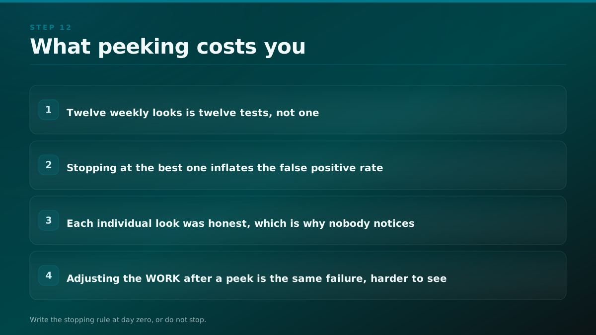
The reason is optional stopping. If you check weekly and stop the moment the gap looks good, you have run twelve tests and reported the most flattering one. That inflates your false positive rate substantially and it does it without anybody lying: each individual look was honest. The permutation test at the end assumes one comparison at one time, and peeking-then-stopping breaks that assumption more thoroughly than any of the sampling problems above.
If you genuinely need an early read, write the stopping rule down at day zero and apply the correction it implies. The cheap version, and the one we would actually recommend, is to not stop.
There is a second-order version of the same failure worth naming, because it is harder to see. Peeking at the readings and then adjusting the WORK is also optional stopping. If week six looks flat and the team responds by pushing harder on the three queries that are closest to flipping, the treated arm is no longer receiving the intervention you are going to describe in the writeup.
Step 13, what this costs
The corpus on this subject is oddly silent about money, so here is the arithmetic in the open.
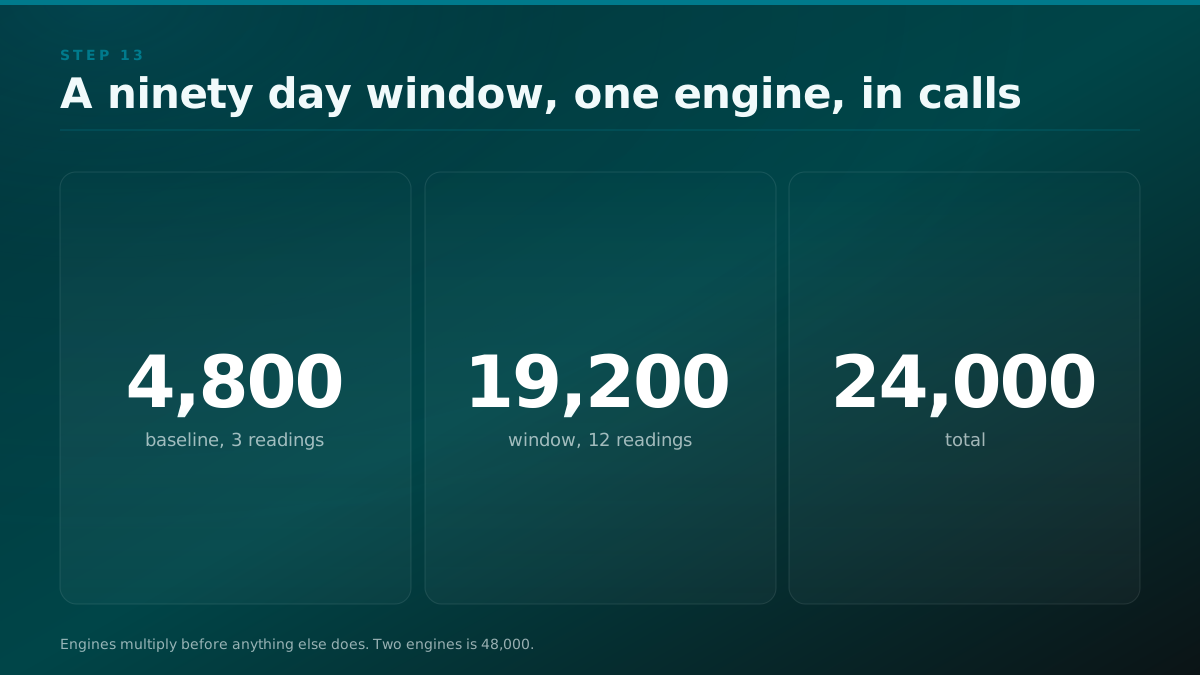
The unit is the assistant call. A 90 day run at weekly cadence on a 40 query by 40 sample design across 1 engine is 40 times 40 times 12 readings, which is 19,200 calls. Add 3 baseline readings at the same size, another 4,800, and you are at 24,000 calls for the window. Two engines doubles it to 48,000 before anything else changes.
At API prices for a mid-tier model with browsing, that is a two to three figure monthly cost, not a four figure one. A practitioner running a thousand prompts at weekly scraping reported a cost of sixty four dollars for that volume, which is the right order of magnitude and a useful sanity check against a tool quote.
The reason tools cost more than the calls is not the calls. It is the storage, the answer parsing, the dashboard and the fact that somebody keeps the engine adapters working when a provider changes its response shape. Those are real costs. They are just not the ones the pricing page implies.
What a 90-day window actually costs in calls
| Component | Calls | Note | Source |
|---|---|---|---|
| Baseline, 3 readings | 4,800 | 40 queries by 40 samples by 3, one engine. | derived |
| Window, 12 weekly readings | 19,200 | Same design, one reading a week. | derived |
| Total, one engine | 24,000 | Derived by addition from the two rows above. | derived |
| Total, two engines | 48,000 | Engines multiply before anything else does. | derived |
as of 2026-09-01
Method: Pure arithmetic from a stated design, so it is derived rather than measured and it is checkable in one line: 40 times 40 times 15 readings is 24,000. Converting calls to money depends on your provider and model and is deliberately not asserted here as a single figure.
Comparing across windows, and the drift you will hit
Once you have two closed windows you will want to compare them, and this is where a well-run programme quietly stops being comparable to itself.
Three things drift between windows and each needs a decision written down.
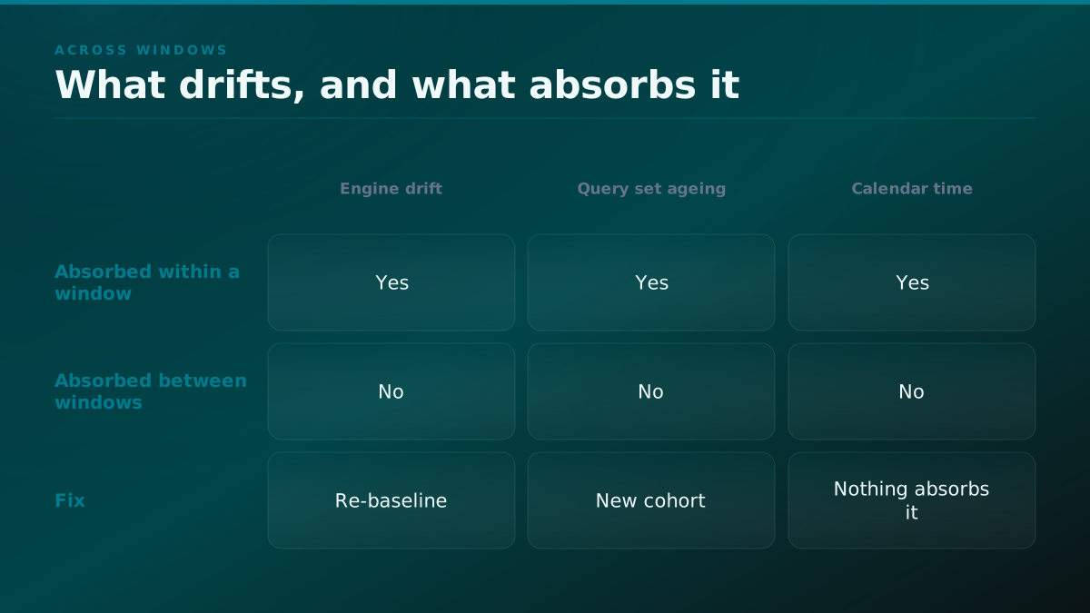
The engine drifts. Model versions change, retrieval behaviour changes, an index refresh lands. Your second window's baseline is not your first window's endpoint. Re-baseline at the start of every window rather than chaining from the previous one, and accept that this costs three readings each time.
The query set ages. Buying language moves, a category term gets adopted, a product you were compared against dies. A frozen set is correct within a window and slowly wrong across a year. Refresh it annually as a new cohort with its own baseline, never by editing the existing set.
The world moves. Competitors publish, a forum thread gets traction. The held-out arm absorbs all of this within a window, which is exactly what it is for, and it absorbs none of it between windows, because there is no control for calendar time.
The consequence is worth stating plainly: a causal claim is a claim about one window. Two windows give you two claims and a trend you can discuss with appropriate hedging. They do not give you a longitudinal measurement, and presenting them as one is the most common way an honest programme starts overclaiming.
Across windows
Three things that drift between windows, and what absorbs them
- Window one resultA causal claim about one window. Valid, and bounded.
- Engine driftModel versions, retrieval behaviour, an index refresh. Re-baseline rather than chain.
- Query set ageingBuying language moves. Refresh annually as a new cohort with its own baseline.
- The world movingCompetitors publish. The held-out arm absorbs this within a window and not between windows.
- Window two resultA second claim, not a continuation of the first.
- Window one resultEngine driftthen
- Window one resultQuery set ageingthen
- Window one resultThe world movingthen
- Engine driftWindow two resultre-baseline
- Query set ageingWindow two resultnew cohort
- The world movingWindow two resultunabsorbed
The one shortcut that is actually safe
If a full window is more than you can commit to, there is a smaller thing that still beats a dashboard reading.
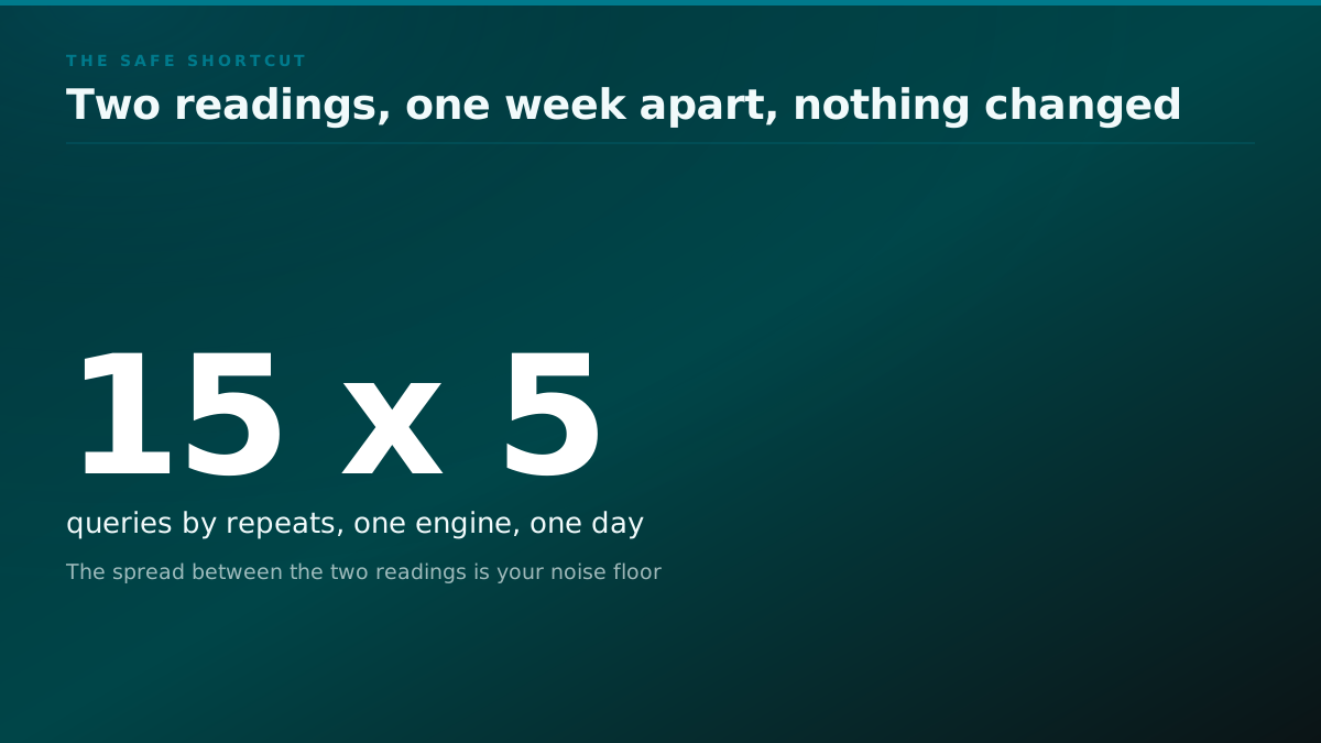
Take fifteen queries. Run each five times, one engine, one day. Compute the proportion per query. Do it again a week later with nothing changed. You now have two readings of a system that by construction should not have moved, and the spread between them is a direct measurement of your own noise floor at almost no cost.
That single number is the thing to hold every future dashboard movement against. It does not give you causality. It gives you the right to say "that is inside our noise" out loud, with a figure behind it, which is most of what this discipline actually buys.
Test the tracker before you trust the tracker
Everything above assumes the instrument does what it says. That is worth ten minutes of checking, because a tracker with a bug reports confidently and a tracker with a bug is indistinguishable from a quiet market.
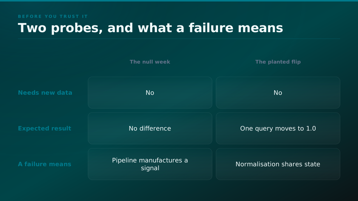
Two probes, both cheap, both of which have to come back the right way.
The null week. Pick a week in which you did nothing at all. Run the full pipeline on it, arms and permutation included. It must report no difference. If it reports one, something in the pipeline is manufacturing a signal, and the usual culprit is that the arm assignment is being recomputed rather than read, so the split is not the split you baselined.
The planted flip. Take one query's stored rows and flip its outcome from not-cited to cited in every repeat. Rerun the reading. The per-query proportion for that one query must go to 1, the arm mean must move by exactly one query's worth, and nothing else must move. If a second query's number changes, your normalisation is sharing state across queries.
Neither probe needs new data. Both run against rows you already have, which is the argument for storing rows.
Before you trust it
Two probes that must come back the right way
- Stored rowsNeither probe needs new data. Both run against rows you already have.
- The null weekA week where nothing was done. The full pipeline must report no difference.
- The planted flipFlip one query to cited in every repeat. That query goes to 1.0 and nothing else moves.
- A trustworthy readingBoth probes had a defined failing result written down first. That is what makes a pass mean something.
- Stored rowsThe null weekreplay
- Stored rowsThe planted flipmutate one query
- The null weekA trustworthy readingreports nothing
- The planted flipA trustworthy readingmoves exactly one
The general shape here is the one thing we would carry from this post into any other measurement work: a check that cannot fail is not a check. Both probes above have a defined failing result, written down before they run, and that is what makes a pass mean something.
Two things that look like signal and are not
Both of these produce a clean, believable move in the treated arm, and both are artefacts.
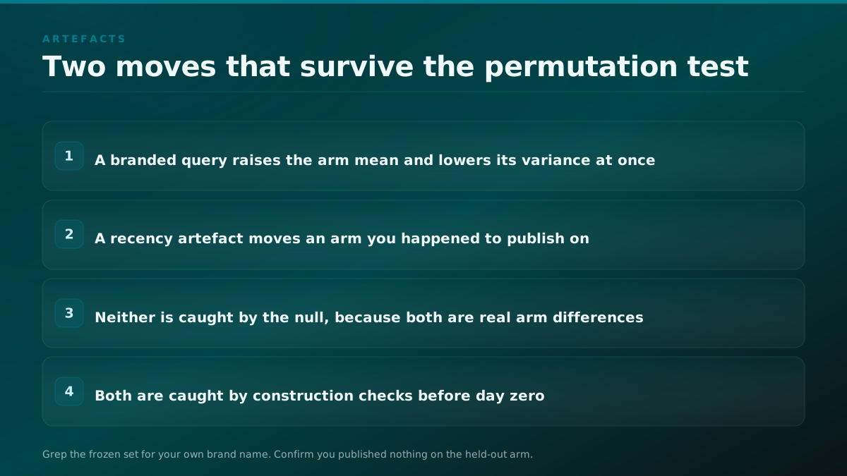
Your own brand name leaking into the query set. A question containing your product name is a question the assistant answers by looking you up, so it will report you cited at a very high rate, stably, forever. It measures existing awareness reflected back. One branded query in a set of twenty raises the arm mean and lowers its variance at the same time, which makes the arm look both better and more precise. Grep the set for your product and company name before day zero.
A recency artefact wearing a lift. Published measurement finds assistants weight recent content, with median cited-content age varying by roughly three months between engines in the same study. If your treated arm is where you happened to publish this quarter, then part of any move you see is the freshness of the pages rather than their content, and it will decay on its own timeline whether or not the work was good. The control arm absorbs this only if you also published nothing on the control arm, which is usually true by construction and worth confirming rather than assuming.
Neither of these is caught by the permutation test, because both are real differences between the arms. They are just not differences your work created. This is the class of error a null distribution cannot see, and it is why the arms have to be comparable in construction and not only in size.
Two artefacts that survive the permutation test
| Artefact | Why the null does not catch it | The check | Source |
|---|---|---|---|
| A branded query in the set | It is a real difference between the arms, just not one your work created. It raises the arm mean and lowers its variance at once. | Grep the frozen set for your product and company name before day zero. | derived |
| A recency artefact | Fresh pages are cited more, so an arm where you happened to publish this quarter moves for reasons that decay on their own timeline. | Confirm you published nothing on the held-out arm, rather than assuming it. | published |
as of 2026-09-01
Method: The branded-query row is derived from the design. The recency row rests on published cross-engine work finding median cited-content age varying by roughly three months between engines, which is somebody else's measurement and is tagged published for that reason.
What this instrument cannot tell you
An honest runbook names its own edges. Here are the four we would raise if you handed us this design and asked what is wrong with it.
It does not attribute revenue. You will have a defensible claim about citation behaviour on a query set. The path from that to a closed deal runs through several steps this instrument does not observe, and anyone who tells you their tool closes that loop is selling you a model, not a measurement.
It does not generalise past your query set. The result is about the queries you froze. If those were not the queries your buyers ask, the measurement is clean and irrelevant. This is why step one is first.
It cannot separate two simultaneous changes. If you shipped documentation and ran a community programme in the same window, the arm difference is the joint effect. Nothing in the maths untangles them. Stagger the work, or accept a joint claim.
It cannot see a model update coming. A silent version change mid-window is a confound that lands on both arms, which the control absorbs, but a version change that interacts with your specific work is not absorbed. Record the version string and be willing to throw a window away.
We have said the negative version of this before, in what predicts an AI citation is not what proves yours, and it is worth repeating in the constructive frame: a large correlational study tells you what associates with citations across pages nobody controls. A controlled two-arm test tells you whether your own work moved your own pages. They are different instruments and neither substitutes for the other.
Scope
What this instrument answers, and what it does not
| A dashboard score | This instrument | Still unanswered by either | |
|---|---|---|---|
| Where do I stand | Yes, as a single collapsed number. | Yes, at four separable levels per engine. | How a buyer weighs what they read. |
| Did my work cause it | No. A change after an action is not an effect. | Yes, within one window, against a null you computed yourself. | Which specific change caused it, if you shipped two at once. |
| Will it hold | No. | No. A causal claim is a claim about one window. | Anything longitudinal, because there is no control for calendar time. |
| Is it worth the money | No. | Partly. It gives you the numerator. | The revenue path, which runs through steps this instrument never observes. |
The failure modes
Nine ways this goes wrong in practice, each one observed in the wild, each one preventable at a specific step.
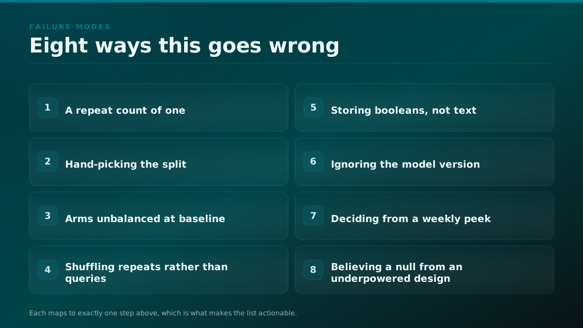
A repeat count of one. No error bar, so no interpretable difference. This is the single most common defect and it is invisible in the output.
Hand-picking the split. The split creates the effect it then measures. Randomise and record the seed.
Unbalanced arms at baseline. Checked in one line before day zero, unfixable at week thirteen.
Shuffling at the wrong level in the permutation. Produces an artificially narrow null and a false result. Shuffle at the unit you randomised.
Storing booleans instead of text. Every metric you did not think of at the time is permanently unavailable.
Ignoring the model version. A silent upgrade reads as your own success.
Running an underpowered pilot and believing its null. The most expensive one, because it produces a confident decision to stop doing work that may have been functioning.
Where this goes wrong, and the step that prevents it
| Failure | Prevented at | Source |
|---|---|---|
| A repeat count of one, so no query carries an error bar | The repeat count decision | derived |
| Hand-picking the split, so the split creates the effect | The held-out arm | derived |
| Arms that started apart at baseline | The baseline balance check | derived |
| Shuffling repeats instead of queries in the permutation | The proof step | derived |
| Storing booleans instead of the answer text | The record schema | derived |
| Ignoring the model version string | The record schema | derived |
| Deciding from a weekly peek before the window closes | The peeking rule | derived |
| Believing a null from an underpowered design | The power arithmetic | derived |
as of 2026-09-01
Method: Derived from failures observed while building and running this instrument, each mapped to the step that would have caught it. It is a checklist rather than a frequency claim: nothing here says how often each one happens.
If you are buying rather than building
The questions to ask a vendor are published. Here is the single test that decides whether anything in this post is available to you at all, and it is not a question about features.
Ask for an export, and look at the shape of a row.
If the export carries one row per query per repeat per engine per reading, with the raw answer text and the source array, you have bought an instrument. Everything above is then yours to run on top of it: the arms, the normalisation, the permutation, the interval.
If the export carries a weekly score per query, or worse a weekly score per account, you have bought a number. No analysis recovers the rows that were thrown away before the export, and the honest description of what you are paying for is a chart rather than a measurement.
That one request separates the two cases in about a minute, and it does it before the contract rather than in month four.
01 / Build the collection layer yourself
- Stands out
- You own the schema, so the four nested observations, the repeat index and the raw answer text are all there from day one. Everything in this post is then available to you.
- Best for
- Teams with an engineer who can spare a day a month and will keep the adapters working when a provider changes its response shape.
- Falls short
- Nobody maintains those adapters but you, and they break on somebody else's release schedule. Also roughly 24,000 metered calls per ninety-day window landing on a card.
02 / Buy a tracker and add the arms on top
- Stands out
- Somebody else owns collection, which is the genuinely hard and genuinely boring part, and you keep the interpretation layer.
- Best for
- Teams who want the presence answer immediately and the causal answer next quarter.
- Falls short
- Entirely dependent on the export. If it carries a weekly score rather than one row per query per repeat, the rows you need were discarded before the export and no analysis recovers them.
03 / Buy the measurement as a service
- Stands out
- The held-out arm is defended by somebody outside the room, which is the failure teams most reliably inflict on themselves under quarterly pressure.
- Best for
- Teams with no engineering time and a real spending decision to make.
- Falls short
- You are trusting somebody else's query set and citation rule. Ask for both in writing before the contract, and ask what their published null looks like.
What the people buying this already say about it
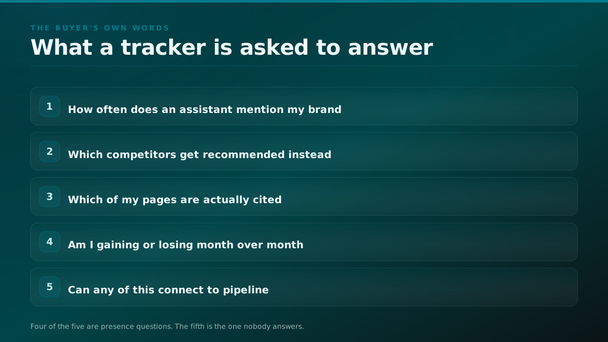
The complaint is consistent enough to be worth reading in the buyer's own words rather than ours. The recurring version is not that the tools are bad, it is that the output is a mention count and the question was whether the mentions did anything.
That thread is a marketer listing the questions a tracker would have to answer to be worth the line item, and every one of them is a question about attribution rather than presence. The category has largely answered the presence question and largely not answered the other one.
The same gap shows up in how the discipline gets taught. Walkthroughs of AI-search measurement tend to cover which metrics exist and where to find them, and stop short of what makes a movement in one of those metrics believable.
None of that is a reason not to buy a tracker. Presence data is genuinely useful and building the collection layer yourself is a real cost. It is a reason to know which of the three questions from the top of this post you are buying an answer to, and to stop expecting the second one to arrive for free with the first.
The order you read the result in
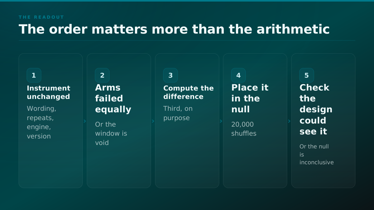
The end of the window is where a well-run measurement most often gets misreported, because the tempting first move is to look at the difference. Do these five in order instead, and stop at the first one that fails.
STEPS
The order you read the result in
First, check the instrument did not move
Two minutes
Same wording, repeat count, engine, normalisation function and model version string across the whole window. If any moved, you are comparing two instruments and there is nothing to read.
Second, check the arms failed equally
Two minutes
Pull per-arm call failure counts. Equal rates are absorbed by the held-out arm. Unequal rates mean an asymmetric shock landed on the comparison and the window is void.
Third, and only now, compute the difference
Seconds
The difference between arm means, per nesting level, per engine. It comes third on purpose: a difference computed before the two checks above is very hard to give up once seen.
Fourth, build the null and place the difference in it
Seconds
20,000 label shuffles at the query level. Report where the observed difference sits, not merely whether it cleared a threshold.
Fifth, build the interval
Seconds
2,000 bootstrap resamples of the queries, repeats kept together, 2.5th and 97.5th percentiles. Report the interval alongside the point estimate.
Last, check the design could have seen a smaller effect
One minute
Compare the observed difference against your minimum detectable lift. If it could not, a null is inconclusive rather than negative, and the honest output is a resized design.
The difference comes THIRD, not first, and that is the whole point of the ordering. A difference computed before the instrument and the failure rates have been checked is a number you will find very hard to give up once you have seen it.
From the field
The teaching material stops where the hard part starts
Walkthroughs of AI-search measurement reliably cover which metrics exist, where to find them and how to read a dashboard. They stop short of what makes a movement in one of those metrics believable: the repeat count, the held-out arm, the null distribution and the power arithmetic. That is not a criticism of the material. It is a map of where the published work currently ends.
The short version
The number on a dashboard is a summary of a summary, and it is not invertible. A reading is a distribution, not a value. A difference is only a result when you know what a difference looks like with nothing done. And a design that cannot detect a plausible win will report your best quarter as a null.
None of that requires a tool. It requires a frozen query set, enough repeats, a held-out half, and the willingness to compute your own noise before you interpret your own signal.
If you want the version of this we run, it is measuring answer engine optimization lift, and the surrounding practice is answer engine optimization.
One last thing, said plainly because it is the part that costs money. The most expensive outcome available here is not a wrong positive. It is an underpowered null: a quarter of real work, measured by a design that could never have seen it, reported as no effect, and used to cancel the programme. That mistake looks exactly like rigour from the outside, which is why the power question belongs at the start of a run and not at the end of one.
Shorter answers to the questions that come up around this procedure, including what actually decides a recommendation and how long before a change can be proved, are collected in the answer feed.
Sources
Every number above, and where it came from. A figure without a row here is one we should not have printed.
- Our own step-zero repeat run, published in the citon corpus
- 12 money queries, 5 identical repeats each, one model, one day, nothing changed between runs. 60 calls, 60 succeeded, 7 of the 12 changed outcome between identical asks. This is the measurement the whole post rests on and it is ours.
- Our own 20,000-split permutation test
- 20,000 random splits of the same query set with no intervention applied. The difference between halves centred on zero, mean plus or minus 0.0016, standard deviation 0.215. The zero mean is the design's kill test; the spread is the bar.
- Our own power analysis for the two-arm design
- Minimum detectable lift by design size: 51.1 percentage points at 12 queries by 5 samples, 21.4 at 20 by 20, 9.9 at 40 by 40. Computed from the variance in our own step-zero run rather than from a vendor table.
- r/aeo, a marketer listing what a tracker would have to answer
- 34 upvotes, 75 comments. The buyer's own framing of the gap this post is about: the tools report presence and the question was attribution. Read live through the Reddit API on 2026-09-01.
- A practitioner's published cost figure for prompt tracking
- 1,000 prompts at weekly scraping quoted at 64 US dollars. Used only as an order-of-magnitude check against our own call arithmetic, not as a price we verified. Read live through the X API on 2026-09-01.
- Search Engine Land, how to measure visibility in AI search
- A walkthrough of which AI-search metrics exist and where to find them. Cited here as evidence for what the teaching material covers, which is collection, and where it stops, which is before interpretation.
Questions people actually ask about tracking AI visibility
- How do you track AI visibility?
- Record four nested observations per answer rather than one score: brand named, anything cited, cited on your own domain, and whether that page was the source the answer leaned on. Ask each query several times rather than once, turn the repeats into a proportion per query, and hold part of the query set back unworked so you have something to compare against.
- How many times should I ask each query?
- Measure it rather than guess. Run ten to fifteen queries five times each on one model on one day and count how many changed outcome. That fraction is your instability rate. Ours was 7 of 12, so 58.3 percent, and at that level three repeats is not enough and five is a floor rather than a target.
- Why does my AI visibility score move when I did nothing?
- Because assistant answers are not stable between identical asks. In our own run, 12 queries repeated 5 times each on one model in one day produced 7 that changed outcome with nothing altered between runs. A single reading is one draw from a distribution, so the movement between two readings is mostly the width of that distribution.
- How do I know whether a change in my AI visibility is real?
- Compare it against the distribution your own data produces when nothing was done. Discard the arm labels, reassign them at random at the query level, recompute the difference, and repeat a few thousand times. Across 20,000 such splits of our own set with no intervention, the null centred on zero with a standard deviation of 0.215, which is the bar a real result has to clear.
- How many queries do I need to detect a real improvement?
- More than most pilots use. Computed from the variance in our own run, a 12 query by 5 sample design has a minimum detectable lift of 51.1 percentage points, 20 by 20 gets to 21.4, 30 by 30 to 11.4 and 40 by 40 to 9.9. Since a real programme moves citation share by single digits to low double digits, only the largest of those designs can see one.
- Should I track ChatGPT, Perplexity and Google together or separately?
- Separately, always. They retrieve differently and they disagree, and a blended number has volatility belonging to none of them. If budget forces a choice, sample one engine properly rather than four thinly, because a well-sampled reading of one supports a claim and four thin ones support none.
- Do I need a tool, or can I build this myself?
- The collection layer is a scheduler, an API key per engine, a table and a few hundred lines. The part worth paying for is somebody maintaining the engine adapters. If you do buy, ask for an export first: if it carries one row per query per repeat you have an instrument, and if it carries a weekly score you have a chart.
Keep reading
Measurement
Prompt Tracking, How Many Prompts and How Many Repeats Before a Change Is Real
Every page ranking for prompt tracking says how to pick prompts. None says how many, or how many repeats, before a weekly change stops being noise.
44 min read
Measurement
Why a single AI visibility score is noise
Twelve money queries, five identical repeats, one model, one day. Seven changed their answer, which breaks every before-and-after published in this category.
24 min read
Measurement
AirOps Alternatives: Content-AEO vs Pure Measurement
Nine real AirOps alternatives, split into content production and pure measurement, plus the buyer split most vendor comparison pages miss entirely.
25 min read